Covariate adjustment in etiologic research:
necessary, but no free lunch
Dr.ir. Richard A.J. Post
When studying an etiologic (study of causes) research question from observational data, most practitioners know they should adjust for confounders. Confounders are features that affect both the outcome and exposure of interest. As a result of the latter, one cannot simply compare the outcomes between groups of individuals with different levels of exposure. An observed difference between the groups will be a mixture of the actual causal effect of the exposure and the effect of the difference (i.e., non-exchangeability) in confounder distribution between the groups. For causal inference, it is thus crucial to balance the levels of these confounders among exposed and unexposed individuals using adjustment methods like stratification, matching, or inverse probability weighting [Chapter 7, 1].
Apart from confounding, spurious correlations can also arise when conditioning on a common cause of the exposure (A) and the outcome of interest (Y). These common causes are called colliders and give rise to a V-structure in causal graphs, as shown in Figure 1. If one would naively adjust for all measured candidate confounders correlated with both the outcome and the exposure, then selection bias is introduced due to the features that are no confounders but colliders and thus also meet this condition. So, one must use expert knowledge to consider what features might be colliders.
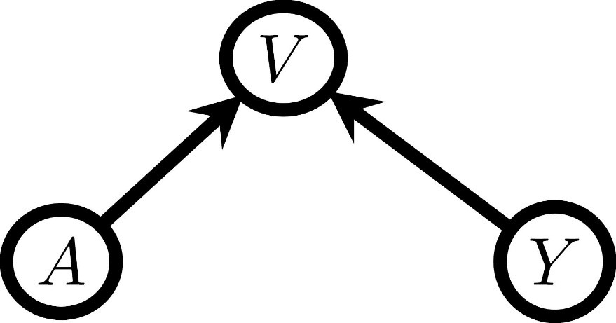
Figure 1
Discussing whether a feature can be a collider is a bit more involved than wondering whether the feature might be caused both by the exposure and the outcome. It is also possible that there are more complicated causal structures, because of which adjustment for a measured feature M introduces selection bias [Chapter 8, 1]. For example, when the exposure and M have an unmeasured common cause U_1, and the outcome and M have an unmeasured common cause U_2, there is a M-structure as shown in Figure 2.
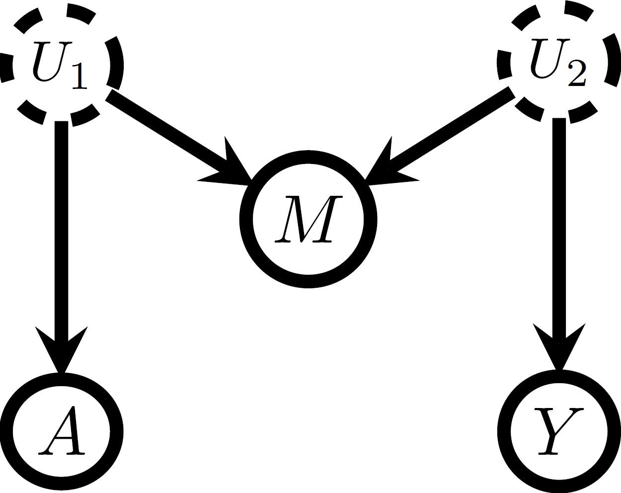
Figure 2
The M-structure has underpinned a longstanding debate in causal inference: “Is it okay to correct for features measured pre-treatment?” [Section 4, 2]. Features measured before treatment can clearly not be colliders in the classical sense since the treatment cannot cause them. However, an underlying M-structure might still exist so that adjustment can result in selection or M-bias. For example, outcome Y can be lung cancer, treatment A taking selective serotonin reuptake inhibitors, while the measured M indicates whether an individual suffers from coronary artery disease, where M is affected by the unmeasured variables depression status (U_1) and smoking status (U_2) [3]. Without adjusting for M, it would become clear that A does not affect Y, but when adjusting for M, a spurious correlation would be found.
In summary, one must not naively include all observed features in a model without carefully thinking about the possible selection bias that can be introduced this way.
References
[1] Hernán MA, Robins JM (2020). Causal Inference: What If. Boca Raton: Chapman & Hall/CRC.
[2] Ding P, Miratrix L (2015). To Adjust or Not to Adjust? Sensitivity Analysis of M-Bias and Butterfly-Bias. Journal of Causal Inference, 3(1), 41-57. https://doi.org/10.1515/jci-2013-0021
[3] Liu W., Brookhart MA, Schneeweiss S, Mi X, Setoguchi S (2012). Implications of M Bias in Epidemiologic Studies: A Simulation Study, American Journal of Epidemiology, 176(10), 938–948, https://doi.org/10.1093/aje/kws165
|